June 2017
Lambertian Reflection Without Tangents
Note (March 2024): This article is somewhat lacking in mathematical rigour but does explain some of the concepts and gives useful details about the presented function itself. I would like to at some point in the near future write a new article putting the idea on firmer theoretical ground.
The Lambert BRDF (after Lambert's cosine law) is pretty ubiquitous in computer graphics. Despite being somewhat nonphysical it agrees with casual observation and produces perceptually-convincing renderings. It's probably the easiest of all the commonly-used BRDFs to understand, to implement, and to calculate. In fact when it is substituted in to the rendering equation it becomes simply the normalising constant 1 / pi. This is because the Lambert reflection function is a cosine lobe - dot(outgoing, normal), and this is already included in the rendering equation - cos(theta). It is view-independent, so it has been very popular as the assumed material BRDF for lightmaps and other types of static baked illumination. For raytracing it is similarly simple to evaluate for Monte Carlo integration with importance sampling. More information about Lambertian reflection can be found here.
vec3 lambert(vec2 uv)
{
float theta = 2 * pi * uv.x;
float r = sqrt(uv.y);
return vec3(cos(theta) * r, sin(theta) * r, sqrt(1 - uv.y));
}
This function produces a reflection vector in the local space of the shading point, with the shading normal as the canonical Z axis. This is nice, but usually it's desired to put the outgoing reflection vector in to world space via a coordinate transformation, and this requires two vectors which are perpendicular to each other and to the shading normal. Here is one possible modification of the function above to do just that:
// This function is based on the CoordinateSystem function from PBRT v2, p63
void CoordinateSystem(in vec3 v1, out vec3 v2, out vec3 v3)
{
if(abs(v1.x) > abs(v1.y))
{
float invLen = 1.0 / length(v1.xz);
v2 = vec3(-v1.z * invLen, 0.0, v1.x * invLen);
}
else
{
float invLen = 1.0 / length(v1.yz);
v2 = vec3(0.0, v1.z * invLen, -v1.y * invLen);
}
v3 = cross(v1, v2);
}
vec3 lambert(vec3 normal, vec2 uv)
{
float theta = 2 * pi * uv.x;
float r = sqrt(uv.y);
vec3 s, t;
CoordinateSystem(normal, s, t);
return s * cos(theta) * r + t * sin(theta) * r + normal * sqrt(1 - uv.y);
}
There are other ways to generate a coordinate system from a single vector. The one used here is from PBRT. Some further information on this is available here. What I will describe in this article is a simple way to calculate the importance-sampled Lambertian reflection vector directly without the need for tangent vectors, and maintaining the same continuous 2D sampling domain.
I used this trick in creating a small pathtraced scene on ShaderToy (it should look like this), because the resulting GLSL code is smaller than it would have been if I had to include code for correctly determining a tangent space transformation.
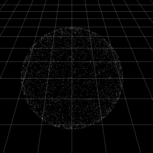
This is the starting point for the method. Points distributed uniformly on the surface of a sphere.
So let's begin with the definitions:
n is the shading normal that you would like to reflect your ray around.
p is a point from a uniform distribution on the surface of the unit sphere, as in the image above.
d is the parallel distance of the point p along the normal.
d = dot(n, p);
Using Archimedes' Hat-Box Theorem it can be determined that points distributed uniformly on a sphere are distributed uniformly when projected on to a line running through the center of the sphere. This is due to the fact that the line can be thought of as a cylinder with radius zero, and the points are distributed uniformly on any cylinder centered around the sphere due to uniform scaling and Archimedes' theorem.
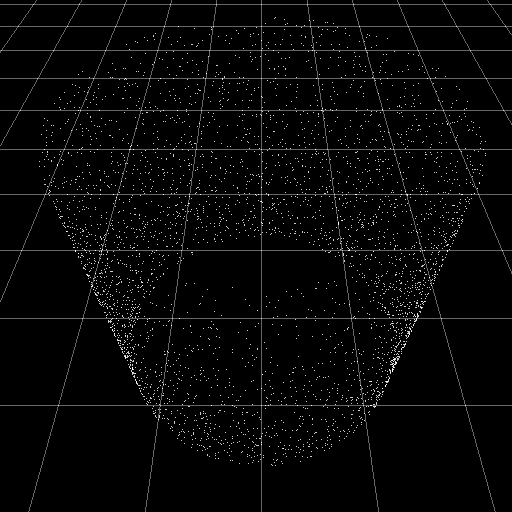
Projecting the points on the sphere onto a cylinder like this results in a uniform distribution of points on the cylinder.
So what is needed is to set the distances of the points from the normal vector according to a mapping which results in a uniform distribution. This can be done by normalizing them (dividing by their length, which is sqrt(1.0 - d * d)) and then setting their distances as sqrt(1.0 - d), which is the normalized inverse CDF (the CDF being the integral of the PDF). The PDF is linear, because each concentric ring in the disc must contain a number of points proportional to the length of the ring, and the length of the ring is a linear function of it's radius (circumference = 2 pi radius). The redistribution needs to occur in a planar fashion so the points are first projected onto the plane defined by the shading normal and the origin. The division by sqrt(2.0) is necessary since d ranges from -1.0 to 1.0 and so the distance remapping extends beyond the unit disc.
p = ((p - d * n) / sqrt(1 - d * d) * sqrt(1 - d)) / sqrt(2);
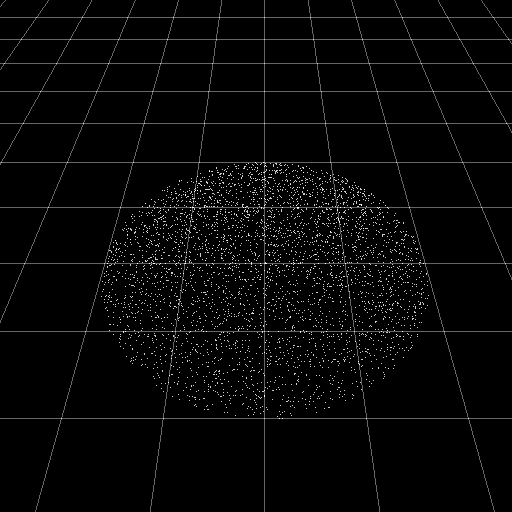
Here the points have been projected onto a plane and redistributed to make them uniform.
After this step the points are distributed uniformly in a disc embedded within a plane defined by the origin and the shading normal n. To then create a sampling point p according to the Lambert BRDF it is only required to project those points on to the hemisphere oriented around the shading normal. This is known as Malley's Method (PBRT v2, p669). dot(p, p) is used here as the squared length of p, of course.
p = p + n * sqrt(1 - dot(p, p));
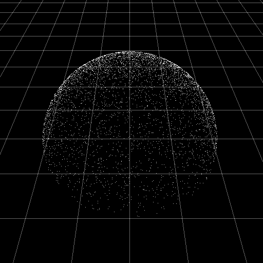
This is the end result of the sampling - a cosine-weighted distribution of points on the unit hemisphere.
After this you have your importance-sampled Lambert reflection. This code is already simple relative to the usual code which generates tangent vectors, but these expressions can be simplified much further.
So the first step is to simplify the scaling term sqrt(2) * sqrt(1 - d) / sqrt(1 - d * d), which becomes simply sqrt(2 + 2 * d). Secondly the dot(p, p) term can be replaced using the knowledge that the resulting length of p will be sqrt(1 - d) / sqrt(2) since it was just set explicitly. That means it can be written as pow(sqrt(1 - d) / sqrt(2), 2), which simplifies to (1 - d) / 2.
p = (p - n * d) / sqrt(2 + d * 2); // Project on to plane and distribute uniformly within the unit disc.
p = p + n * sqrt(0.5 + d / 2); // Project on to the unit hemisphere. Simplified from sqrt(1 - (1 - d) / 2).
These two steps can be combined together by collecting terms:
p = p / sqrt(2 + d * 2) + n * (sqrt(0.5 + d / 2) - d / sqrt(2 + d * 2));
It turns out that (sqrt(0.5 + d / 2) - d / sqrt(2 + d * 2)) can be simplified to 1 / sqrt(2 + d * 2) so this statement can be simplified to:
p = p / sqrt(2 + d * 2) + n / sqrt(2 + d * 2);
And then obviously:
p = (p + n) / sqrt(d * 2 + 2);
So the final simplified and tidy GLSL function looks like this:
vec3 lambertNoTangent(vec3 normal, vec2 uv)
{
float theta = 2 * pi * uv.x;
uv.y = 2 * uv.y - 1;
vec3 spherePoint = vec3(sqrt(1.0 - uv.y * uv.y) * vec2(cos(theta), sin(theta)), uv.y);
return (normal + spherePoint) * inversesqrt(dot(normal, spherePoint) * 2 + 2);
}
And it can also be optimized a little:
vec3 lambertNoTangent(in vec3 normal, in vec2 uv)
{
float theta = 6.283185 * uv.x;
uv.y = 2 * uv.y - 1;
vec3 spherePoint = vec3(sqrt(1.0 - uv.y * uv.y) * vec2(cos(theta), sin(theta)), uv.y);
return normalize(normal + spherePoint);
}
Without Normalizing
If it's not necessary for the resulting vector to be normalized, then things get even simpler. The result becomes a set of points on the unit sphere offset by the shading normal, basically a sphere sitting on the surface being shaded. This isn't so surprising if you consider this diagram which shows in 2D that the rays form a circle, and the fact that the Lambert BRDF is isotropic so in 3D the rays form a sphere.
vec3 lambertNoTangentUnnormalized(vec3 normal, vec2 uv)
{
float theta = 2 * pi * uv.x;
uv.y = 2 * uv.y - 1;
vec3 spherePoint = vec3(sqrt(1.0 - uv.y * uv.y) * vec2(cos(theta), sin(theta)), uv.y);
return normal + spherePoint;
}
Results
Shown below is a comparison between the standard method of computing the reflection vector in worldspace via tangent vectors derived via axis-flips, and my direct method described above. The scene is just a typical raytraced bunch of spheres on a plane, and the shading done by taking 1024 samples of ambient occlusion.
So in addition to being a smaller amount of code and free of discontinuities (and in my opinion more mathematically pure), it can also provide a small performance improvement. In fact in my tests the function turns out to be faster than the branch-free version used in this ShaderToy shader from iq (check out the cosineDirection function).
To see the code in action, check it out on ShaderToy.

